Intro to R

Basics of R

R is a versatile, open source programming/scripting language that’s useful both for statistics but also data science. Inspired by the programming language S.

• Free/Libre/Open Source Software under the GPL.
• Superior (if not just comparable) to commercial alternatives. R has over 7,000 user contributed packages at this time. It’s widely used both in academia and industry.
• Available on all platforms.
• Not just for statistics, but also general purpose programming.
• For people who have experience in programmming: R is both an object-oriented and a so-called functional language.
• Large and growing community of peers.

Presentation of RStudio

Let’s start by learning about RStudio, the Integrated Development Environment (IDE) that we will use to write code, navigate the files found on our computer, inspect the variables we are going to create, and visualize the plots we will generate. RStudio can also be used for other things (e.g., version control, developing packages) that we will not cover during the workshop.

RStudio is divided into 4 “Panes”: the editor for your scripts and documents (top-left), the R console (bottom-left), your environment/history (top-right), and your files/plots/packages/help/viewer (bottom-right). The placement of these panes and their content can be customized.

R as a calculator

The lower-left pane (the R “console”) is where you can interact with R directly. The > sign is the R “prompt”. It indicates that R is waiting for you to type something.

You can type Ctrl + Shift + 2 to focus just on the R console pane. Use Ctrl + Shift + 0 to get back to the four panes. I use this when teaching but not otherwise.

Let’s start by subtracting a couple of numbers.

2016 - 1969

## [1] 47

R does the calculation and prints the result, and then you get the > prompt again. We won’t discuss what that number might mean. (The [1] in the results is a bit weird; you can ignore that for now.)

You can use R as a calculator in this way.

4*6
4/6
4^6
log(4)
log10(4)
log(4, 10)
log(4, 6)

Here log is a function that gives you the natural logarithm. Much of your calculations in R will be through functions. The value in the parentheses is called the function “argument”. log10 is another function, that calculates the log base 10. There can be more than one argument, and some of them may have default values. log has a second argument base whose default (the value if left unspecified) is e.

?log

Need for Scripts

We can go along, typing directly into the R console. But there won’t be an easy way to keep track of what we’ve done.

It’s best to write R “scripts” (files with R code), and work from them. And when we start creating scripts, we need to worry about how we organize the scripts and data for a project.

And so let’s pause for a moment and talk about file organization.

Creating an R Project

It is good practice to keep a set of related data, analyses, and text self-contained in a single folder, called the working directory. All of the scripts within this folder can then use relative paths to files that indicate where inside the project a file is located (as opposed to absolute paths, which point to where a file is on a specific computer). Working this way makes it a lot easier to move your project around on your computer and share it with others without worrying about whether or not the underlying scripts will still work.

RStudio provides a helpful set of tools to do this through its “Projects” interface, which not only creates a working directory for you but also remembers its location (allowing you to quickly navigate to it) and optonally preserves custom settings and open files to make it easier to resume work after a break. Below, we will go through the steps for creating an RProject for this tutorial.

• Start RStudio (presentation of RStudio -below- should happen here)
• Under the File menu, click on New project, choose New directory, then Empty project
• Enter a name for this new folder (or “directory”, in computer science), and choose a convenient location for it. This will be your working directory for the rest of the day (e.g., ~/data-carpentry)
• Click on “Create project”
• Under the Files tab on the right of the screen, click on New Folder and create a folder named data within your newly created working directory. (e.g., ~/data-carpentry/data)
• Create a new R script (File > New File > R script) and save it in your working directory (e.g. data-carpentry-script.R)

Your working directory should now look like this:

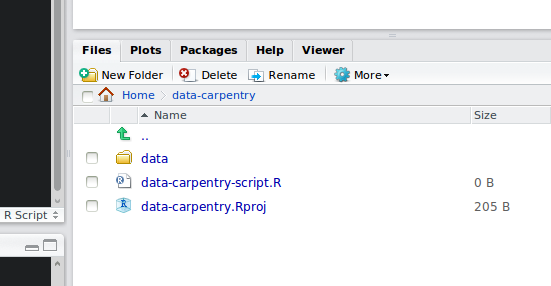
How it should look like at the beginning of this lesson

Organizing your working directory

Using a consistent folder structure across your projects will help keep things organized, and will also make it easy find/file things in the future. This can be especially helpful when you have multiple projects. In general, you may create directories (folders) for scripts, data, and documents.

• data/ Use this folder to store your raw data and intermediate datasets you may create for the need of a particular analysis. For the sake of transparency and provenance, you should always keep a copy of your raw data accessible and do as much of your data cleanup and preprocessing programmatically (i.e. with scripts, rather than manually) as possible. Separating raw data from processed data is also a good idea. For example, you could have files data/raw/tree_survey.plot1.txt and ...plot2.txt kept separate from a data/processed/tree.survey.csv file generated by the scripts/01.preprocess.tree_survey.R script.
• documents/ This would be a place to keep outlines, drafts, and other text.
• scripts/ This would be the location to keep your R scripts for different analyses or plotting, and potentially a separate folder for your functions (more on that later).

You may want additional directories or subdirectories depending on your project needs, but these should form the backbone of your working directory. For this workshop, you only need a data/ folder.

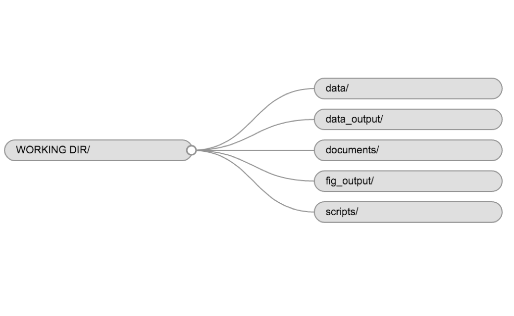
Example of a working directory structure

Interacting with R

While you can type R commands directly at the > prompt in the R console, I recommend typing your commands into a script, which you’ll save for later reference, and then executing the commands from there.

Start by typing the following into the R script in the top-left pane.

# R intro

2016 - 1969

Save the file clicking the computer disk icon, or by typing Ctrl + S.

Now place the cursor on the line with 2016 - 1969 and type Ctrl + Enter. The command will be copied to the R console and executed, and then the cursor will move to the next line.

You can also highlight a bunch of code and execute the block all at once with Ctrl + Enter.

Assignment operator

We can assign names to numbers and other objects with the assignment operator, <-. For example:

age <- 2016-1969

Type that into your script, and use Ctrl + Enter to paste it to the console.

You can also use = as assignment, but that symbol can have other meanings, and so I recommend sticking with the <- combination.

In RStudio, typing Alt + - will write <- in a single keystroke.

If you’ve assigned a number to an object, you can then use it in further calculations:

sqrt(age)

## [1] 6.855655

You can assigned that to something, and then use it.

sqrt_age <- sqrt(age)
round(sqrt_age)
round(sqrt_age, 2)

Object names

Objects can be given any name such as x, current_temperature, or subject_id. You want your object names to be explicit and not too long.

They cannot start with a number (2x is not valid, but x2 is).

R is case sensitive (e.g., weight_kg is different from Weight_kg). There are some names that cannot be used because they are the names of fundamental functions in R (e.g., if, else, for, see here for a complete list).

In general, even if it’s allowed, it’s best to not use other function names (e.g., c, T, mean, data, df, weights). In doubt check the help to see if the name is already in use.

It’s also best to avoid dots (.) within a variable name as in my.dataset. There are many functions in R with dots in their names for historical reasons, but because dots have a special meaning in R (for methods) and other programming languages, it’s best to avoid them. It is also recommended to use nouns for variable names, and verbs for function names. It’s important to be consistent in the styling of your code (where you put spaces, how you name variable, etc.). In R, two popular style guides are Hadley Wickham’s and Google’s.

x <- 50
y <- x * 2
x <- 80

Objects in your workspace

The objects you create get added to your “workspace”. You can list the current objects with ls().

ls()

RStudio also shows thee objects in the Environment panel.

Vectors and data types

A vector is a group of values, mainly either numbers or characters. You can assign this set of values to a variable, just like you would for one item. For example we can create a vector of animal weights:

weights <- c(30, 100, 4000, 8000)

A vector can also contain text (character strings):

animals <- c("rat", "cat")

There are many functions that allow you to inspect the content of a vector. length() tells you how many elements are in a particular vector:

length(weights)
length(animals)

An important feature of a vector, is that all of the elements are the same type of data. The function class() indicates the class (the type of element) of an object:

class(weights)
class(animals)

The function str() provides an overview of the object and the elements it contains. It is a really useful function when working with large and complex objects:

str(weights)
str(animals)

You can add elements to your vector by using the c() function:

animals <- c(animals, "dog") # adding at the end of the vector
animals <- c("mouse", animals) # adding at the beginning of the vector

What happens here is that we take the original vector animals, and we are adding another item first to the end of the other ones, and then another item at the beginning. We can do this over and over again to grow a vector, or assemble a dataset. As we program, this may be useful to add results that we are collecting or calculating.

We just saw 2 of the 6 atomic vector types that R uses: "character" and "numeric". These are the basic building blocks that all R objects are built from. The other 4 are:

• "logical" for TRUE and FALSE (the boolean data type)
• "integer" for integer numbers (e.g., 2L, the L indicates to R that it’s an integer)
• "complex" to represent complex numbers (e.g. 1+4i)
• "raw" that we won’t discuss further

Vectors are one of the many data structures that R uses. Other important ones are lists (list), matrices (matrix), data frames (data.frame) and factors (factor).

x <- c(1, 2, 3, 'a')

y <- c(1, 2, 3, TRUE)

z <- c('a', TRUE, 'b', 'c')

tricky <- c(1, '2', 3, 4)

Subsetting vectors

If we want to extract one or several values from a vector, we must provide one or several indices in square brackets. For instance:

animals <- c("mouse", "rat", "dog", "cat")
animals[2]

## [1] "rat"

animals[c(1, 4)]

## [1] "mouse" "cat"

We can also repeat the indices to create an object with more elements than the original one:

more_animals <- animals[c(1, 2, 3, 2, 1, 4)]

R indexes start at 1. Programming languages like Fortran, MATLAB, and R start counting at 1, because that’s what human beings typically do. Languages in the C family (including C++, Java, Perl, and Python) count from 0 because that’s simpler for computers to do.

animals <- c("mouse", "rat", "dog", "cat")

x <- c(21, 54, 39, 17, 55)
x[c(FALSE, TRUE, FALSE, FALSE, TRUE)]

## [1] 54 55

x > 50    # will return logicals with TRUE for the indices that meet the condition

## [1] FALSE  TRUE FALSE FALSE  TRUE

## so we can use this to select only the values above 50
x[x > 50]

## [1] 54 55

x[x < 30 | x > 50]

## [1] 21 54 17 55

x[x > 30 & x < 50]

## [1] 39

animals <- c("mouse", "rat", "dog", "cat")
animals[animals == "cat" | animals == "rat"] # returns both rat and cat

## [1] "rat" "cat"

animals %in% c("rat", "cat", "dog", "duck")

## [1] FALSE  TRUE  TRUE  TRUE

animals[animals %in% c("rat", "cat", "dog", "duck")]

## [1] "rat" "dog" "cat"

animals <- c("mouse", "rat", "cat", "dog")
weights <- c(30, 180, 4000, 8000)

Missing data

As R was designed to analyze datasets, it includes the concept of missing data (which is uncommon in other programming languages). Missing data are represented in vectors as NA.

heights <- c(2, 4, 4, NA, 6)

When doing operations on numbers, most functions will return NA if the data you are working with include missing values. It is a safer behavior as otherwise you may overlook that you are dealing with missing data. You can add the argument na.rm=TRUE to calculate the result while ignoring the missing values.

mean(heights)
max(heights)
mean(heights, na.rm = TRUE)
max(heights, na.rm = TRUE)

If your data include missing values, you may want to become familiar with the functions is.na() and na.omit(). examples.

## Extract those elements which are not missing values.
heights[!is.na(heights)]
## shortcut to that
na.omit(heights)

v <- c(2, 4, 4, "NA", 6)
mean(v, na.rm=TRUE)